The tutorial here represents the absolute basics of using the BioDeepTime database. More elaborate tutorials will be made available on Evolv-ED.
Add toc: true to the metadata of the .md file for a table of contents.
The Data
Download
The BioDeepTime database is made available through the ‘chronosphere’ research data API. The R client to access data can be installed from the CRAN servers with:
install.packages("chronosphere") # used to call the data
install.packages("tidyverse") # used for data manipulation and plotting
install.packages("ggrepel") # used for plotting
The most up-to-date version of the denormalized BioDeepTiem database can be accessed with:
# attach package
library(chronosphere)
Chronosphere - Evolving Earth System Variables
Important: never fetch data as a superuser / with admin. privileges!

Note that the package was split for efficient maintenance and development:
 - Plate tectonic calculations -> package 'rgplates'
 - Arrays of raster and vector spatials -> package 'via'
library(tidyverse)
── Attaching core tidyverse packages ──────────────────────── tidyverse 2.0.0 ──
✔ dplyr     1.1.2     ✔ readr     2.1.4
✔ forcats   1.0.0     ✔ stringr   1.5.0
✔ ggplot2   3.4.2     ✔ tibble    3.2.1
✔ lubridate 1.9.2     ✔ tidyr     1.3.0
✔ purrr     1.0.1

── Conflicts ────────────────────────────────────────── tidyverse_conflicts() ──
✖ dplyr::collapse() masks divDyn::collapse()
✖ tidyr::fill()     masks divDyn::fill()
✖ dplyr::filter()   masks stats::filter()
✖ dplyr::lag()      masks stats::lag()
✖ dplyr::slice()    masks divDyn::slice()
ℹ Use the conflicted package (<http://conflicted.r-lib.org/>) to force all conflicts to become errors
library(ggrepel)

# download data, verbose=FALSE hides the default chatter
bdt <- fetch("biodeeptime", verbose=FALSE)
Note that this table is rather large and might take a bit of time to
load. The accessible data items can be downloaded with
(datasets("biodeeptime")).
Structure
The default representation of the denormalized table is a data.frame,
where every row represents one record or biogeographic observation (the
presence of a taxon in a sample).
str(bdt)
'data.frame':   7437847 obs. of  39 variables:
 $ db                : chr  "Neotoma" "Neotoma" "Neotoma" "Neotoma" ...
 $ seriesID          : chr  "TS_1" "TS_1" "TS_1" "TS_1" ...
 $ seriesOriginalName: chr  "Konus Exposure, Adycha River" "Konus Exposure, Adycha River" "Konus Exposure, Adycha River" "Konus Exposure, Adycha River" ...
 $ seriesOriginalID  : chr  "11" "11" "11" "11" ...
 $ long              : num  136 136 136 136 136 ...
 $ lat               : num  67.8 67.8 67.8 67.8 67.8 ...
 $ depthUnit         : chr  "cmbct" "cmbct" "cmbct" "cmbct" ...
 $ ageModel          : chr  "4" "4" "4" "4" ...
 $ reason            : chr  "Community analysis" "Community analysis" "Community analysis" "Community analysis" ...
 $ sampleID          : chr  "S_1" "S_1" "S_1" "S_1" ...
 $ sampleOriginalID  : chr  "158" "158" "158" "158" ...
 $ sampleOriginalName: chr  NA NA NA NA ...
 $ depth             : num  0 0 0 0 0 0 0 0 0 0 ...
 $ age               : num  1321 1321 1321 1321 1321 ...
 $ ageProc           : chr  "bchron" "bchron" "bchron" "bchron" ...
 $ ageOld            : num  2463 2463 2463 2463 2463 ...
 $ ageYoung          : num  355 355 355 355 355 ...
 $ timeOriginalUnit  : chr  "Radiocarbon years BP" "Radiocarbon years BP" "Radiocarbon years BP" "Radiocarbon years BP" ...
 $ timeOriginal      : num  1000 1000 1000 1000 1000 1000 1000 1000 1000 1000 ...
 $ timeOriginalOld   : num  NA NA NA NA NA NA NA NA NA NA ...
 $ timeOriginalYoung : num  NA NA NA NA NA NA NA NA NA NA ...
 $ waterDepth        : num  NA NA NA NA NA NA NA NA NA NA ...
 $ preservation      : chr  NA NA NA NA ...
 $ samplingEffort    : num  NA NA NA NA NA NA NA NA NA NA ...
 $ minimumMesh       : num  NA NA NA NA NA NA NA NA NA NA ...
 $ maximumMesh       : num  NA NA NA NA NA NA NA NA NA NA ...
 $ environment       : chr  "Terrestrial or Freshwater" "Terrestrial or Freshwater" "Terrestrial or Freshwater" "Terrestrial or Freshwater" ...
 $ samplingEffortType: chr  NA NA NA NA ...
 $ totalCount        : num  809 809 809 809 809 809 809 809 809 809 ...
 $ taxonID           : int  4 10 3 11 8 1 13 12 5 9 ...
 $ analyzedTaxon     : chr  "Valeriana" "Onagraceae" "Ericaceae" "Cyperaceae" ...
 $ species           : chr  NA NA NA NA ...
 $ genus             : chr  NA NA NA NA ...
 $ openNomenclature  : chr  NA NA NA NA ...
 $ analyzedRank      : chr  NA NA NA NA ...
 $ group             : chr  "Plants" "Plants" "Plants" "Plants" ...
 $ abundance         : num  2 6 2 7 5 1 22 12 3 5 ...
 $ abundanceUnit     : chr  "count" "count" "count" "count" ...
 $ refID             : chr  "2" "2" "2" "2" ...
 - attr(*, "chronosphere")=List of 13
  ..$ dat         : chr "biodeeptime"
  ..$ var         : chr "denormalized"
  ..$ res         : logi NA
  ..$ ver         : num 1
  ..$ datafile    : chr "biodeeptime.rds"
  ..$ item        : int 702
  ..$ reference   : chr "Jansen A. Smith, Marina C. Rillo, Ádám T. Kocsis, Maria Dornelas, David Fastovich, Huai-Hsuan M. Huang, Lukas J"| __truncated__
  ..$ bibtex      : chr "@misc{jansen_a_smith_2023_8154672,\n author = {Jansen A. Smith and\nMarina C. Rillo and\nÁdám T. Kocsis and\nMa"| __truncated__
  ..$ downloadDate: POSIXct[1:1], format: "2023-07-20 09:51:33"
  ..$ publishDate : chr "2023-07-12"
  ..$ infoURL     : logi NA
  ..$ API         : logi NA
  ..$ additional  : list()
Basic analyses
The number of time series in the database:
length(unique(bdt$seriesID))
[1] 10062
The number of records in the database:
length(bdt$db)
[1] 7437847
The number of unique sampling locations:
nrow(unique(bdt[, c("long", "lat")]))
[1] 8752
The oldest record (relative to 1950) in each database:
bdt %>% group_by(db) %>% summarize(max = max(age))
# A tibble: 9 × 2
  db                               max
  <chr>                          <dbl>
1 BioTIME                         49.4
2 Direct uploads             1146200
3 Geobiodiversity Database 451050000.
4 MARBEN                    77200000
5 Neotoma                   23900000
6 Neptune SandBox          151075752
7 Paleobiology Database    150889174.
8 SedTraps                       -28.4
9 Triton                    65997000
Finding the mean age (relative to 1950) of a sample from modern databases (BioTIME and SedTraps):
modern <- bdt %>%
  filter(db == "BioTIME" | db == "SedTraps") ## filtering to only modern data

mean(modern$age)
[1] -44.50505
Finding the mean age (relative to 1950) of a sample from fossil databases:
fossil <- bdt %>%
  filter(db != "BioTIME" & db != "SedTraps") ## filtering to exclude modern data

mean(fossil$age)
[1] 5087525
For additional analyses and visualization, data summarization and manipulation can be done as follows:
## this manipulation summarizes information for each unique time series
overview <- bdt %>%
  group_by(seriesID) %>%
  dplyr::summarise(db = unique(db), ## source database
                   #environment = unique(environment), ## broadly defined environment
                   group = unique(group), ## taxonomic group
                   lat = unique(lat), ## latitude
                   long = unique(long), ## longitude
                   #abundType = unique(abundanceUnit), ## abundance type of records
                   samples = length(unique(sampleID)), ## number of samples
                   richness = length(unique(analyzedTaxon)), ## number of unique species
                   meanAge = mean(age, na.rm = TRUE), ## mean age of samples
                   minAge = min(age, na.rm = TRUE), ## minimum age of a sample
                   maxAge = max(age, na.rm = TRUE), ## maximum age of a sample
                   extent =  maxAge - minAge) ## temporal extent (duration) of the time series
Warning: Returning more (or less) than 1 row per `summarise()` group was deprecated in
dplyr 1.1.0.
ℹ Please use `reframe()` instead.
ℹ When switching from `summarise()` to `reframe()`, remember that `reframe()`
  always returns an ungrouped data frame and adjust accordingly.

`summarise()` has grouped output by 'seriesID'. You can override using the
`.groups` argument.
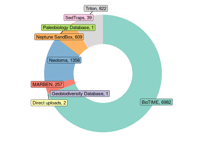
Visualizing the data
Create a donut plot showing the contribution of source databases to BioDeepTime:
## donut plot for proportion contribution of each database
databases <- overview %>%
  group_by(db) %>%
  dplyr::summarise(count = n())

# Compute percentages
databases$fraction <- databases$count / sum(databases$count)

# Compute the cumulative percentages (top of each rectangle)
databases$ymax <- cumsum(databases$fraction)

# Compute the bottom of each rectangle
databases$ymin <- c(0, head(databases$ymax, n=-1))

# Compute label position
databases$labelPosition <- (databases$ymax + databases$ymin)/2

# Compute a good label
databases$label <- paste0(databases$db, ", ", databases$count)

# # Make the plot
ggplot(databases, aes(ymax=ymax, ymin=ymin, xmax=4, xmin=3, fill=db)) +
   geom_rect() +
   geom_label_repel(x = 4, aes(y=labelPosition, label=label), size=4) + ## x controls label position (inside/outside donut)
   scale_fill_brewer(palette = "Set3") +
   coord_polar(theta="y") +
   xlim(c(2, 4)) +
   theme_void() +
   theme(legend.position = "none") ## controls the presence of a legend